Quantum Teleportation with Qiskit
Starting with the disillusion, quantum teleportation is not really about actually teleporting stuff from one place to another in the common sense of the word. In fact, I’d rather call it quantum replication, since the point is to replicate the state of a qubit in a different qubit somewhere else using information received from classical channels; meaning that the transfer of information is still bounded by the speed of light. So, if you want to send your hypothetical state to the nearest star, Proxima Centauri, you’d still have to wait about 4 years for the information to get there via this protocol.
Now, I have seen plenty of implementations of a quantum teleportation circuit in several tutorials. Some of them, completely go over the fact that you’re not supposed to know the state of the qubit you’re teleporting at the receiver’s end. This means that adding a “disentangler” gate at the end of the circuit that uses information about how you prepared the state in the first place trivializes the whole process.
In short, here’s how the quantum teleportation protocol works:
Encoding
- First, you prepare the quantum qubit that you would like to teleport, say $|\psi\rangle = \alpha |0\rangle + \beta |1 \rangle$.
- You prepare an entangled pair of qubits, one of which you keep with you and the other you send to the receiver.
- You entangle your qubit and the entangled qubit you have kept with yourself.
- You measure your qubits. By now, the states have collapsed into two classical bits (00 to 11) and a quantum bit.
- The bits you have obtained in the previous step are also sent to the receiver, in the form of a string for example (
01).
Decoding
- The receiver will apply an X gate to his entangled state if he gets a string that begins with 1, and a Z gate if he gets a string that ends with 1.
- The resulting amplitudes can be recovered via an ensemble method.
Now, an attentious reader would notice that the receiver cannot know what was the phase of the complex coefficients $\alpha$ and $\beta$ were via this protocol. He can merely find you what their absolute values are. The reason for that, is simply because measuring the state $| \psi \rangle$ give you no information about its phase, only its amplitude squared. To this point, you might argue that we don’t end up with the same state at the receiver’s end, and that’s technically correct, the best kind of correct.
With that out of the way, we can start thinking about the actual implementation. We will use the Qiskit library along with Qiskit Aer to simulate the circuit locally. You could, in principle, run this on a real quantum computer via the IBM API, but this code is so simple that it feels wasteful to do so.
Implementation
from qiskit import __version__
from qiskit_aer import __version__

print("Qiskit version: ", __version__)
print("Qiskit Aer version: ", __version__)
Qiskit version:  0.14.1
Qiskit Aer version:  0.14.1
Encoding and Preparation
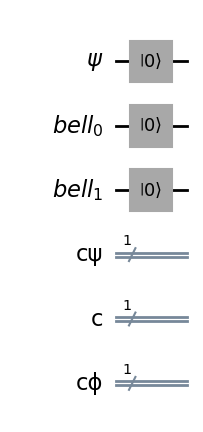
We start by initializing our circuit. We will need a total of 3 qubits and 3 classical bits. The QuantumRegister and ClassicalRegister objects are just conveniences to help us keep track of which qubit (or classical bit) is which. If you don’t like, you could instantiate the quantum circuit directly with QuantumCircuit(3, 3).
import numpy as np
from qiskit import QuantumCircuit, QuantumRegister, ClassicalRegister

# Register qubits and classical bits
ψ = QuantumRegister(1, 'ψ')
cψ = ClassicalRegister(1, 'cψ')

bell = QuantumRegister(2, 'bell')
c = ClassicalRegister(1, 'c')
cϕ = ClassicalRegister(1, 'cϕ') #This will be used to read the final result

# Create a quantum circuit
qc = QuantumCircuit(ψ, bell, cψ, c, cϕ)
qc.reset(ψ)
qc.reset(bell)

qc.draw(output='mpl') #Needs pylatexenc, you can also just call .draw() to get a text representation
Now, we will prepare the qubit we want to send. This is done with a series of operations that end up with the configuration that you want.
from qiskit.quantum_info.states.random import random_statevector
from qiskit.circuit.library import Initialize

#Generate two random complex numbers
random_vec = random_statevector(2)

#We will store the squared probabilities for future reference
probs = np.abs(random_vec)**2
probs = {0: probs[0], 1: probs[1]}

state = Initialize(random_vec)
qc.append(state, ψ)

qc.draw(output='mpl')
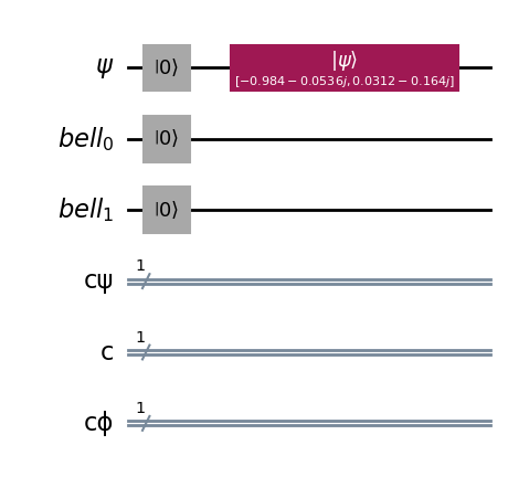
#Peeking at the expected probabilities

probs
{0: 0.972049603070859, 1: 0.027950396929141353}
The next step is to prepare out Bell state. This will output an entangled state of two qubits. The standard way to do this is to apply a Hadamard gate to the first qubit and then a CNOT gate with the first qubit as the control and the second qubit as the target.
The process works like this:
- Start with zeroes. This is just a choice and you could start with any other state.
- Apply the Hadamard gate to the first qubit.
- Apply CNOT gate.
So at the output of the bell qubits, we expect it to be either $|00\rangle$ or $|11\rangle$ with equal probability.
qc.h(bell[0])
qc.cx(bell[0], bell[1])

qc.barrier() #This is just for visualization purposes

qc.draw(output='mpl')
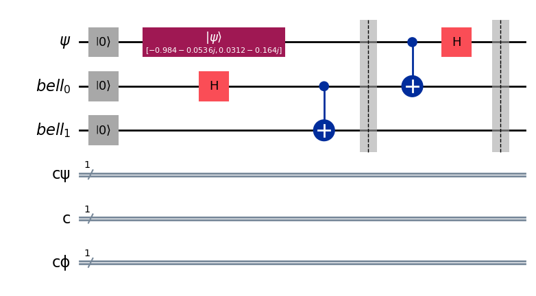
Now, we will entangle the qubit we want to send with the first qubit of the Bell state. This is done by applying a CNOT gate with the qubit we want to send as the control and the first qubit of the Bell state as the target and then applying a Hadamard gate to the qubit we want to send.
Mathematically this becomes:
- State after Bell entanglement:
or
\[\frac{\alpha}{\sqrt{2}}|000\rangle + \frac{\alpha}{\sqrt{2}}|011\rangle + \frac{\beta}{\sqrt{2}}|100\rangle + \frac{\beta}{\sqrt{2}}|111\rangle\]- Apply CNOT gate.
or
\[\frac{\alpha}{\sqrt{2}}|0\rangle \otimes \left(|0\rangle \otimes |0\rangle + |1\rangle\otimes|1\rangle \right) + \frac{\beta}{\sqrt{2}}|1\rangle \otimes \left(|1\rangle \otimes |0\rangle + |0\rangle\otimes|1\rangle \right)\]- Apply Hadamard gate and simplify
Notice how what ends up in the parentheses has the same amplitude we want to send with some phase. The first term is exactly what we want to send, the second one has the bits 0 and 1 flipped (solvable by an X gate), the third one needs to change the sign of 1 (using a Z gate), and the latter has both the bits flipped and the sign changed (solvable by a ZX gate).
qc.cx(ψ, bell[0])
qc.h(ψ)

qc.barrier()
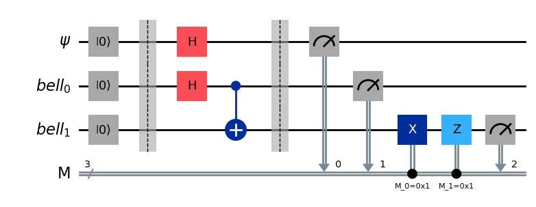
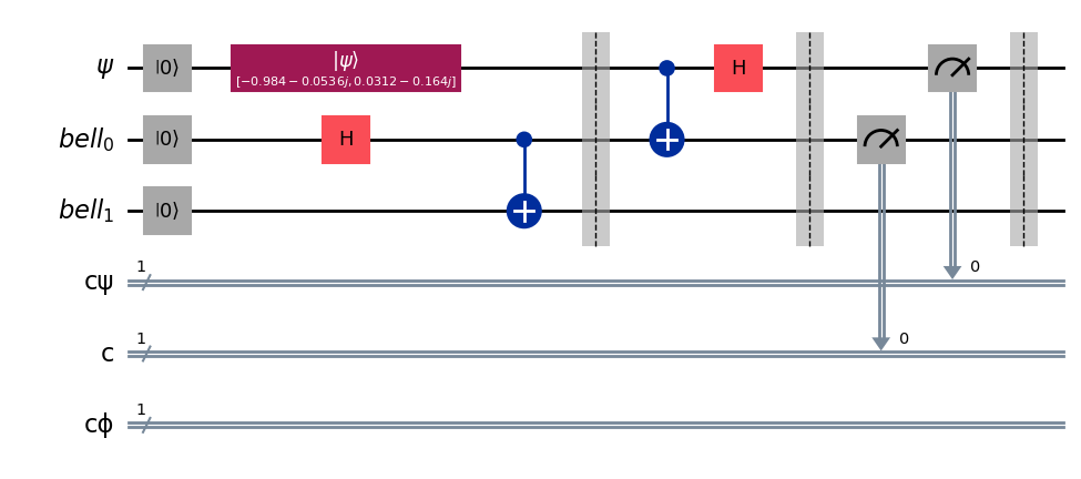
Finally, we read the outcome of out prepared qubit and the first entangled qubit to send it to the receiver.
qc.measure(bell[0], c)
qc.measure(ψ, cψ)
qc.barrier()

qc.draw(output='mpl')
Decoding
Once the receiver got the measurements made earlier along with the second entangled state (bell_1). We can move on to the deconding process. The procedure is as follows:
| Received | Gate Applied |
|---|---|
| 00 | I |
| 01 | X |
| 10 | Z |
| 11 | ZX |
Notice that the order of the operations is inverted when we actually apply the gates. So, the ZX gate actually means to apply the X gate followed by the Z gate.
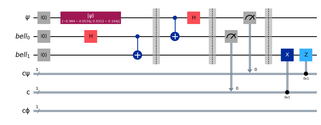
Luckly, we can encode this whole process with the .c_if method of Qiskit. You can think of it as the same as a controlled gate, except that the control is a classical bit. So, if the classical bit is 1, the gate is applied, otherwise it is not.
qc.x(bell[1]).c_if(c, 1)
qc.z(bell[1]).c_if(cψ, 1)

qc.draw(output='mpl')
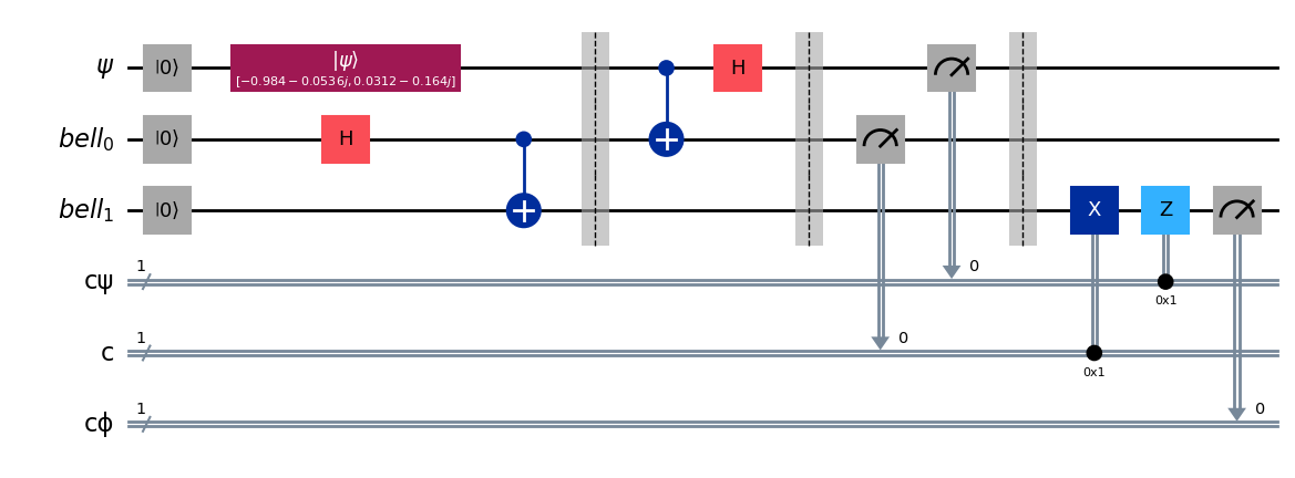
Reading out the Outcome with Ensemble Statistics
One way to find out whether our protocol is working is via an ensemble method. The idea revolves in running this code many times over and then checking the statistics of the outcomes. If the protocol is working, we should see that the outcomes are $|0\rangle$ and $|1\rangle$ with the same probability that we started with (the probs) variable.
#Measure the final state
qc.measure(bell[1], cϕ)

qc.draw(output='mpl')
from qiskit_aer import AerSimulator

simulator = AerSimulator()
result = simulator.run(qc, shots=10000).result()

print(result.get_counts())
{'1 1 0': 65, '1 0 1': 69, '1 0 0': 73, '0 0 1': 2341, '0 0 0': 2453, '0 1 0': 2465, '1 1 1': 55, '0 1 1': 2479}
In oder to make things humanly readable, we will focus only on the third bit, which is the one we are actually reading in the receiveing end. The other two bits are due to the intermediate measurements we made to prepare the qubit.
probs
{0: 0.972049603070859, 1: 0.027950396929141353}
from collections import Counter

receiver_counts = Counter()
receiver_counts = Counter()
for k, v in result.get_counts().items():
    receiver_counts[k[0]] += v/1000 #The order is inverted, so the first bit is the last one
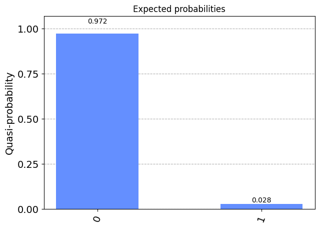
Now, we should see the distributions of the outcomes to be fairly close to the probs variable. You can run this code multiple times to see how the distributions change.
from qiskit.visualization import plot_histogram

plot_histogram(receiver_counts, title='Receiver probabilities')

plot_histogram(probs, title='Expected probabilities')
Link to notebook: Quantum Teleportation